➤How to use the IF function in Excel? 🕹

Excel is a tool with which we can perform a plethora of calculations, from the simplest to the most complicated.

In this tutorial, we focus on Excel's IF function. Each formula is illustrated by an example of a situation but of course it adapts to the needs of each one.

What is the IF function?

Indicated price:

The IF function is used to determine whether a condition is met or not, and if it is not then another condition, created by the user, is provided.

In summary, it allows to make logical comparisons between a value and the expected result. This function can therefore have two results because if the first result is true then it must be applied. If it is not then the 2nd one will be.

The logical formula is Si a datum is true, then let's apply this solution, otherwise let's apply another solution. For example, if he raining, then close the windows, otherwise leave them open.

The Excel syntax or structure of this IF formula looks like this: =IF(logical_test, value_if_true, value_if_false).

Delay notices

Indicated price:

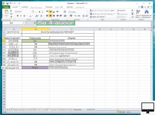
In our first worksheet, a company's accountant needs to check whether each payment was received on the due date or not.

The due date is listed in column A, the payment status is listed in column B, and the customer name is listed in column C.

1/In column A, cell A1, enter the formula: =TODAY(), to display the current date.

2/ In column B, cell B4, enter the formula: IF(A4-TODAY()>30;"Late";"OK").

It will be used to determine which customers are in arrears of more than 30 days.

In other words, the formula means: Si the date in cell A4 minus today's date is greater than 30 days, then enter "Late" in cell B4, otherwise, enter "OK".

3/All you have to do is drag your cursor from cell B4 to cell B13 to apply the formula everywhere.

Pass/Fail Internal Training

Indicated price:

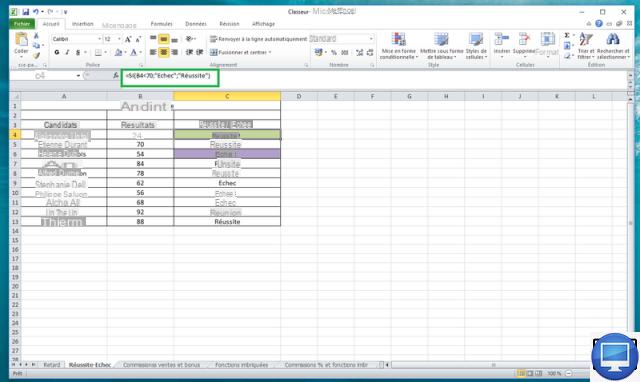
To complete internal training, employees must pass a test.

Candidates who total a score below 70% fail the exam, if it is higher then they pass it.

1/ In column A, list the names of all the candidates.

2/ In column B, report their result.

3/ In column C, the success or failure of the exam will be displayed. This information is obtained using the SI function.

4/ In cell C4, enter the formula: = SI (B4 <70; "Echec"; "Réussite").

It means that si the result in cell B4 is less than 70 then enter "Failed", otherwise enter "Success".

Now all you have to do is drag your cursor to cell C13.

Nested IF functions

Indicated price:

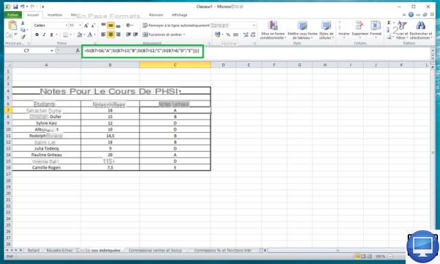
In this example, we will convert numbered exam scores to letters using nested SI formulas. This consists of joining several functions in the same formula.

The names of the students are entered in column A, their grades in B and their equivalent in letters, calculated using the SI functions, will be in column D.

We entered in cell C7, the following formula:

=SI(B7>16;"A";SI(B7>13;"B";SI(B7>12;"C";SI(B7>8;"D";"E"))))

Then just drag your cursor to the last cell in the table.

Note: Note that each open parenthesis must be closed at the end of the function.

Sales commissions and bonuses

Indicated price:

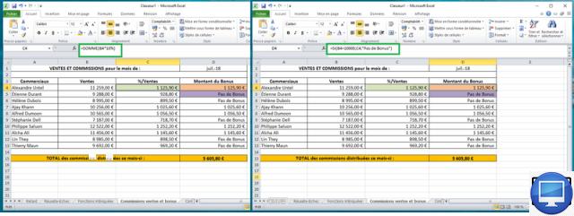
Wilcox companies pay 10% commission to their marketing team if they manage to achieve more than 10 euros in sales. If the amount is lower then she does not receive a bonus.

1/ Enter in column A the name of each member of the marketing team.

2/ In column B, enter the total amount of sales made during the month.

3/ In column C, multiply the total sales by 10%, i.e. =SUM(B4*10%). Drag the slider from C4 to C13.

4/ Finally, in column D enter the formula =IF(B4>10000;C4;"No Bonus").

It will then be displayed the amount of the commission in €, if it is greater than €10, or "No Bonus".

Then slide your cursor from D4 to D13.

5/ Now, to calculate the total bonuses, enter in the column D15 =SUM(D4:D13) and press the key Starter.

Percentage commissions and nested functions

Indicated price:

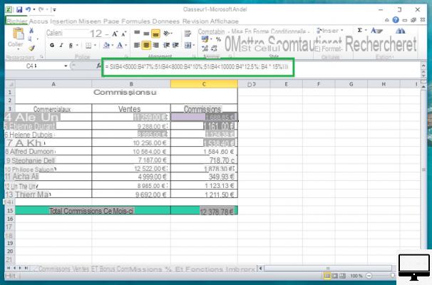
In this example, we'll use another nested IF function technique. This makes it possible to calculate several percentages of commissions, then to make the totals of these monthly commissions.

1/ In column A, is the name of the members of the marketing team.

2/ In column B is reported each total amount of sales made over the month.

3/ In column C, the commissions are entered.

4/ In cell C4, enter the following formula: =SI(B4<5000;B4*7%;SI(B4<8000;B4*10%;SI(B4<10000;B4*12,5%;B4*15%)))

5/ Finally in cell C15, the total amount calculated automatically with the SI function will be entered.

Enter in C15, the formula: = SUM (C4: C13).

Price of a product calculated on the basis of the quantity

Indicated price:

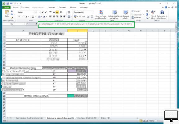
Many resellers, and especially wholesalers, give their customers a quote based on the quantity of products.

For example, a wholesaler might sell 1-10 T-shirts at $10,50, and 11-25 T-shirts at $8,75.

Use the following formula to determine how much you will save by purchasing products in bulk:

1/ Name the cell A3 Wholesale price, cell B3 Quantity and cell C3 Cost.

2/ From B4 to B9, enter the different quantities and their respective prices in column C.

3/ Now, create a second table with the products for sale (A12 to A18), the ordered quantity (B12 to B18).

4/ Finally, name the cell C11 Cost per quantity and in the cell just below, enter the formula:

=B13*SI(B13>=101;3,95;SI(B13>=76;5,25;SI(B13>=51;6,3;SI(B12>=26;7,25; SI(B13>=11;8;SI(B13>=1;8,5))))))

5/ Finally, enter in the cell for the total amount: = SUM (C13: C19).

If your prices and quantities change, all you have to do is enter this data, Excel will adjust the formulas and calculations.

Use other formulas in the IF function

Indicated price:

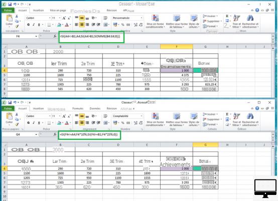
In this example, we will nest 2 IF functions and insert the SUM formula into them. The goal is to determine if a person's goals are less than, equal to, or greater than those of the company.

1/ Enter in cell B1 theMonthly Goal. It can be changed monthly to reflect business expectations.

2/ Name the cells A3 to G3 as follows: Objectives, 1er Trim, 2nd Trim, 3ème Trim, 4ème Trim, Objectiveset Bonus.

3/ From cell A4 to A8, enter the goals of the top 5 members of the marketing team.

4/ Finally, enter the quarterly totals for each salesperson, from cell B4 to cell E8.

Those who have reached their sales targets will earn 10% bonus of the total amount in euros.

For those who have exceeded them, the bonus will be 25%.

Here is how to calculate, respectively, the objectives and the bonuses in €:

5/ Enter cell F4, =SI(A4<=B1,A4,SI(A4>B1,SOMME(B4:E4,0))) and drag it to cell F8.

6/ Then, in cell G4, enter: =SI(F4<=A4,F4*10%,SI(F4>=B1,F4*25%,0)) and drag it to G8.

Use the IF function to avoid dividing by zero

Indicated price:

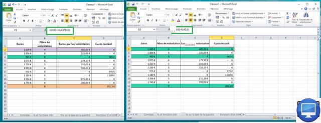
In Excel, when you try to divide a number by zero, the error message appears: #DIV/0!.

So what if you have a large database that requires divisions, and some cells contain the number zero? The solution is the IF function.

1/ To calculate the money collected each month by the volunteers of the charity organization, (which we invented) Espoir et Vie, name 4 columns of your table as follows: A1 euros, B1 No. (number) of volunteers, C1 Euros by volunteers and D1 Euros remaining.

The amount entered in column A will then be divided between each volunteer.

The number of volunteers can be 0 because some days the organization is closed.

2/ In cell C2, up to C11, enter: =SI(B2<>0.A2/B2.0). You will see that thanks to the IF function, it is possible to divide your amounts by zero.

3/ In cell D2, copy the formula = SI (B4 = 0; A4; 0) and drag it to D11. If there is no volunteer, then no money will be donated.

4/ Now go to B2 and enter = MAX (B2: B11), this is used to identify the maximum number of volunteers, which is 8.

5/ Finally, in cell D12 type =SUM(D2:D11)/B12.
In total, the 8 volunteers will share €392,50.