➤Excel drop-down list: create, insert, modify, delete 🕹

To make it easier to type into your Excel spreadsheets, use simple or dynamic drop-down lists that adapt to your data. You will avoid errors and your data will be more homogeneous.

Want to avoid entering the same data all the time in Excel? Prevent typing errors? Standardize the entry of labels to make aggregations more easily? There are a thousand and one good reasons to use drop-down lists to enter data into Microsoft's spreadsheet software! With two clicks in the spreadsheet, all you have to do is select the right value from a list.

The principle of the drop-down list is simple: it consists of offering ready-made choices in a "drop-down menu", by preparing various options and by setting some rules. It is the simplest and most efficient solution, both for data entry and for the consistency of data and titles.

Excel is teeming with good ideas and input help to make your life easier. Here are several methods, very simple or more sophisticated, to display drop-down lists and validate the data entered by yourself or by the users of your spreadsheets. Good news: these techniques work with almost all versions of Excel, even older ones, on both Windows and Mac, sometimes with a few nuances that we specify.

How to use Excel's autocomplete list?

Let's start with the easiest way, where Excel takes care of everything. It's probably already doing you a favor in Windows and Mac; there is just a keyboard shortcut to know to be sure to take full advantage of it.

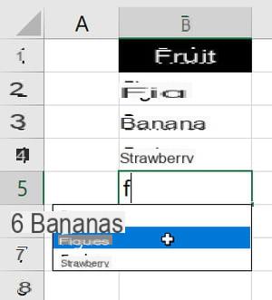
Type a few letters in a cell of a column already containing elements: Excel suggests one or more values already entered in the same column. It's here autocomplete.

Excel drop-down list: create, insert, modify, delete

If the list does not appear, type the keyboard shortcut Alt + Down Arrow (the arrow of the four arrow keys). This two-key combination causes Excel to display the list so you can select a value that has already been entered.

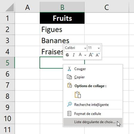
You can also right click on the cell to choose Drop-down list of choices in the context menu, which will show you the list.

Excel displays an empty or incomplete list if one or more empty cells are listed above in the column. While you can type a space in these cells so that they are no longer empty, the trick may affect your calculations, for example if you use the COUNTA function to find out how many items your column has. Up to you…
This drop-down list only works for text, not for numeric values or dates, and only if the data is in columns. Excel removes the duplicates and sorts the values alphabetically before presenting the list to you.
To turn off autofill in Excel for Windows, go to File> Options> Advanced options (in the left column), and under the section Edit options, uncheck the box Autocomplete cell values.
To configure Excel for Mac, go to Excel menu> Preferences> Auto-complete.

How to create drop down list with data validation in Excel?

Thanks to the data validation function, Excel can check for you what the user enters in a cell, and not authorize; for example, only numbers, or only a date between two limits, or a caption - of 15 characters maximum - or even a value drawn from a list that you are going to specify: this is exactly what interests us here.

With data validation, the user retains the right to type a value in the cell rather than selecting it from your drop-down list. But you can refuse any unexpected value entered, or display a warning before finally accepting the entered value. Here is the principle for creating a drop-down list.

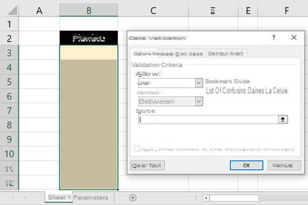
Select the cells where the user should scroll the list to enter data more easily (here B3: B12).
In the Excel ribbon, click the tab Data then Data validation.
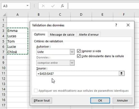
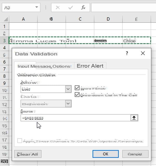
In the zone To allowchoose List.
Leave the boxes checked Ignore if empty et Drop-down list in cell.

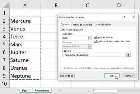
Click in the area Source then select in your worksheet the range of cells containing the list to display (here the range of cells A2: A9 of the sheet that we have called Parameters).
press OK and test your drop-down list by clicking in one of the cells that should display this list.

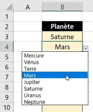
In the worksheet, visually, there is nothing to indicate that a drop-down list is provided for input. It is only when you select the cell that a small icon appears on the right, which must be clicked to expand the list.
To scroll the list, you can also press the combination of two keys Alt + Down Arrow.
Below we give you some tips for preparing your list of items to display.
When you select the cell or range of cells where your drop-down list should appear, select the entire column if necessary by clicking on its letter in the grid, for example on C to select the entire column C (it will be easy to exclude it then only certain cells, for example C1 and C2, via the button Reset all of the dialog box Data validation).

The area Source - which indicates where the list of items to display is located - accepts different types of information: text, a range of cells, a named zone, a formula… We are going to discover all the subtleties of this Source zone.

A tip in Excel for Windows: when you click in the box Source and you want to move inside to modify its content, press (once) the key F2 before using the Left / Right arrow keys on the keyboard.

How to create drop down list with fixed values in Excel?

This method is suitable if the list has only a handful of values, which are not likely to change.

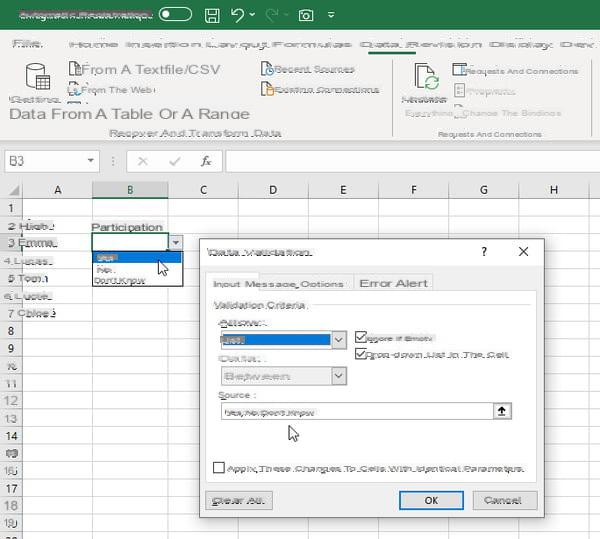
After choosing Data> Data validation> Authorize> List, in the zone Source, type values separated by semicolons (or by commas if you are in an English version of Excel), without spaces between the values, for example the three choices: Yes; No; Don't know
Be careful, with this type of Source, Excel distinguishes between upper and lower case (we say that it takes "case" into account). So if the user types YES in the cell instead of selecting Yes from the drop-down list, Excel will return an error message (see Error Alerts below). The other methods explained below are not case sensitive.

How to create drop down list in Excel from range of cells?

This method is useful when the list can contain many entries and when it does not change or rarely.

After choosing Data> Data validation> Authorize> List, click in the area Source then click in a sheet to select with the mouse or the keyboard a range of cells, in row or in column.

You can of course also type the range of cells in the box yourself. Source.
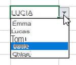
When you then type a value instead of choosing it from the drop-down list, Excel ignores upper and lower case letters. If the value Lucie is in your list, the user will be able to type lucie, LUCIE or LuCie in the cell without receiving an error message.

We explain how to add or remove items from the source list below without having to change the Data Validation for that drop-down list.

How to make drop down list in Excel from named range?

This method has several advantages: the list can be very long; names always make formulas more understandable, and by using a formula to define the scope of the named cell range, the drop-down list will automatically adapt to changes when adding or removing items.

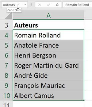
To name a range of cells in Excel, first select those cells and then click in the box Name, just above column A, and type the name: in our example, we selected the cell range A4: A10 and typed Authors, which becomes the name of the range. A name can only start with the letters A to Z or with the _ sign and must not contain spaces (see the tab Packages > Name manager for other options).

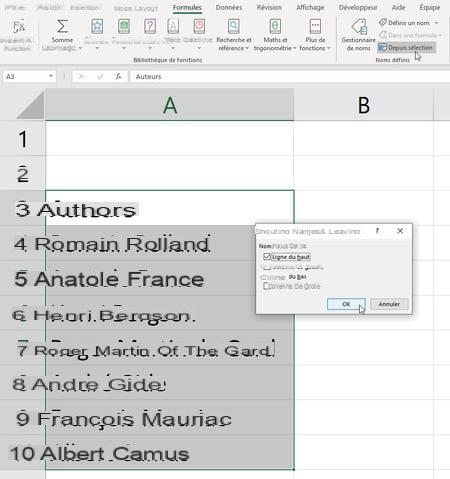
Another even simpler method to name a range when the first cell of that range already has a title: select cells with this column header, here our title is Authors, so select cells A3: A10 and, in the tab Packages, click on From a selection. Check that the box Top line (and only it) is checked and press OK. The range A4: A10 (therefore without the first title cell) is named with the content of the first selected cell (here A3), the range A4: A10 is therefore called here Authors. If cell A3 contained the text French Auteurs, the name would be Auteurs_français because in the named ranges, spaces and hyphens are replaced in the name by signs _ by Excel.
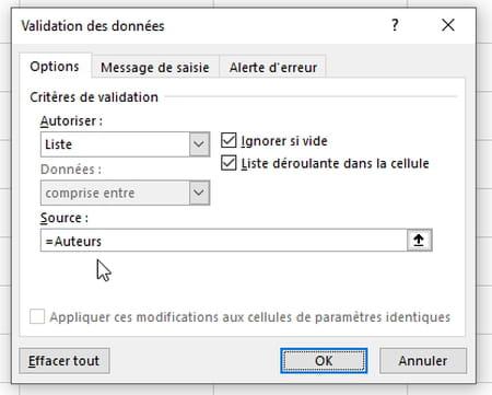
Select the cells where the drop-down list should be displayed and click on the tab Data> Data validation> Authorize> List.
In the window Data validation, For Source from your list, type the = (equals) sign followed by the name of the named range, so = Authors in our example.

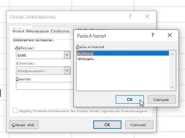
Instead of typing the name of the track, when editing the contents of the Source area, you can also press the key. F3 in Excel for Windows: the small window Paste a name pops up, it lists all the named areas in your workbook. Click on the name that interests you, here Authors, Excel adds the formula = Authors in the zone Source.

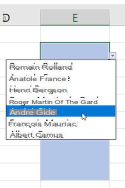
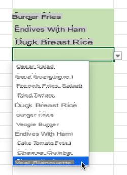
Here is our drop-down list in which you just need to pick an author.

We explain later how to add or how to remove items from your source list without having to reconfigure the drop-down list.

How to make dynamic drop down list from table in Excel?

With this method, when you add or remove data from the source list, the drop-down list automatically adapts to reflect the changes. Other methods allow it, this one has the merit of elegance and clarity, in particular because all the ranges of cells on which you work are named. And Excel "tables" have many other advantages.

Click one of the source data cells or select the entire range of cells with its column names. Your table can have one or more columns, the drop-down list will only use one column anyway, which you will specify later by name.

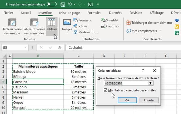
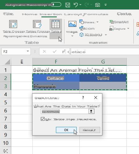
Under the tab Insertion, click on Table.
If you had not selected the entire table, Excel selects the data it believes should be part of the table, including column titles (headers). Check that the selection is right for you.
Check the box My table has headers and press OK. In our example, our headers are Aquatic Mammals and Size.

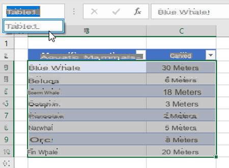
Excel names Table1 the first table created in the workbook (ignore the drop-down lists it adds to the right of the headers). Check the table name by clicking in the upper left corner in the box Name. Click on the name to select the entire table: Table1 does not take the headers into account (it therefore covers B3: C10 in our example), but Excel keeps them preciously in memory ...
Now select the cells where the entry drop-down list should appear.
Click on the tab Data> Data validation> Authorize> List.
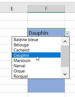
In the zone Source, type = INDIRECT ("TableName [column header]") ie = INDIRECT ("Table1 [Aquatic mammals]") in our example.
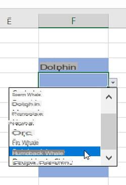
Test your drop-down list ...

At the end of the source list, add one or more items in the empty cells. Below, we type two new items, Humpback Whale and Chinese Dolphin, at the end of the list ...

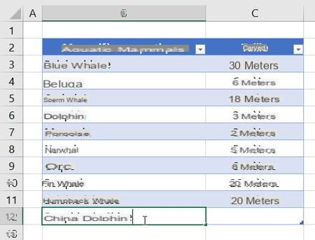
… Automatically, our Table1, which spanned B3: C10, now covers the range of cells B3: C12. And without having to do anything, the drop-down list takes into account the two added items.

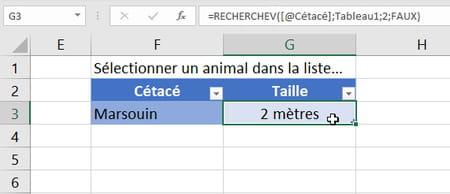
Would you like to display the size of the animal when you select one from the list? In the entry sheet, enter headers just above the drop-down list (Cetacean and Size, on our example) then select this mini table (headers and first row of data) and click on Insertion, Table to create this time a Table2.

In G3, enter the formula = VLOOKUP ([@ Cetacean]; Table1; 2; FALSE)
The size of the animal selected just to the left in the drop-down list is automatically displayed ...

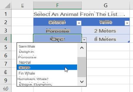
When you are at the end of this table, here in cell G3, press the key Tab on your PC or Mac keyboard to add a row to the Table2 table. In cell F4, the drop-down list is copied and at your disposal to select an animal, choose one from the list and its size will automatically be entered in cell G4, since the formula entered in G3 is also , automatically copied to G4.

To adapt our formula = VLOOKUP ([@ Cetacean]; Table1; 2; FALSE) to your data, here are some explanations:
► the VLOOKUP function searches for a value in the first column to the left of an array (here in Table1), and returns a value on the same row of the array, but from another column
► @ Cetacean is the text that we typed in F2 and which here becomes a header of Table2, it points to the text you are looking for in Table1 (here the name of the animal entered in the cell using the list drop down)
► Table1 is the table in which the search is therefore carried out
► the value "2" corresponds to the column number where the value that must be returned is located (here the second column of Table1, which includes the size of the animals)
The value FALSE is important, do not omit it, it specifies here that you want an exact search for the name of the animal, and not the closest value (otherwise indicate the value TRUE, but in this case the list of names animals must be sorted in ascending order).
Finally, some commands to know to manage tables ... If you prefer to remove the small drop-down lists that appear in the headers of the source table: tab Home> Sort and Filter> Filter.

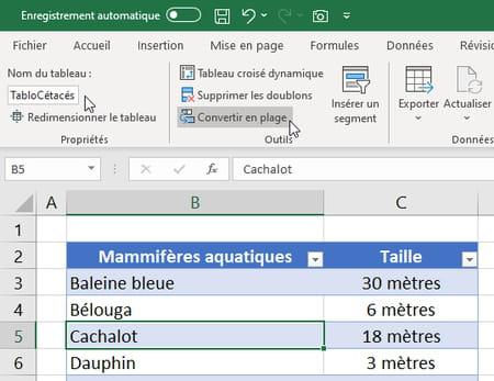
To rename a table, click on one of its cells, click on the tab Table creation which pops up to the far right of the ribbon (after File, Home, Insertion, Layout…), then rename the table at the top left of the screen (here Table1 is renamed TabloCetaceans). To delete a table, click Convert to range (the contents of the cells are preserved).

How to create drop down list from Excel formula?

With this method, if you add items to the source list, they automatically appear in the drop-down list. We propose here a relatively "simple" formula, but all the power of Excel is at your disposal to define the source elements of your list. And, as we will see, a name can also be associated with a formula rather than a range of cells ...

Once your data has been entered in column, select the cells where the drop-down list should appear and click on the tab Data> Data validation> Authorize> List.

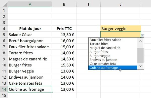
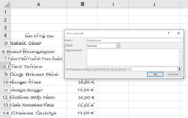
In the zone Source, with the data from our example above, type the formula = OFFSET ($ A $ 5; 0; 0; COUNT ($ A: $ A) -1; 1)
And here is our list ...

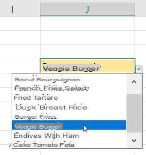
If you add a new item at the end of the source list (below Cheese Quiche), it is automatically added to the drop-down list.

This formula = OFFSET ($ A $ 5; 0; 0; COUNT ($ A: $ A) -1; 1) will be easy to adapt to your own data:
► the OFFSET function returns a reference to a range of cells (explanations here) which contain the list to display;
► $ A $ 5 refers to the first cell of our source list;
► leave 0; 0; to apply no horizontal or vertical offset;
► $ A: $ A corresponds to the column (A) where the source list is located;
► COUNTA counts the number of non-empty cells in this column (here the result is 11);
► value -1: we subtract 1 from the number returned by NBVAL (11 in our example) because one of our cells contains a list header (Daily special), which should not be taken into account;
► the last 1 corresponds to the number of columns of the reference returned by OFFSET (leave the value 1).
You could very well associate this formula with a name. Let's first see how to do it in Windows ...

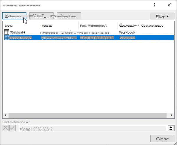
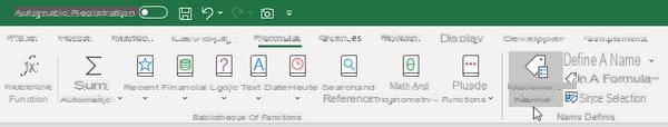
In Windows, regardless of the currently selected cell: click on the tab Packages then Name manager, then the button New.
Give your list a new name, for example PlatsDuJour (without spaces, and the first letter must be a letter from A to Z or the underscore _).

In the zone Refers to, copy-paste the formula seen above, i.e. = OFFSET ($ A $ 5; 0; 0; COUNT ($ A: $ A) -1; 1)
Press the OK button and close the Data manager window.

Now let's see how to perform the same manipulation On Mac.

To associate a formula with a name, regardless of the cell selected, click on the tab Packages then Define a name.
Type the new name, here PlatsDuJour (spaces are prohibited and the name must start with a letter from A to Z or the underscore _).

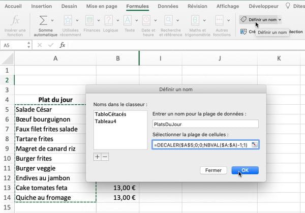
In the zone Select range of cells, copy-paste the formula = OFFSET ($ A $ 5; 0; 0; COUNT ($ A: $ A) -1; 1)
Press the button OK.
In Windows or macOS, now select the cells where the drop-down list should appear. Click on the tab Data then Data validation.

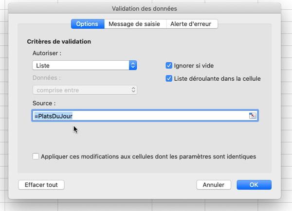
Choose Allow> List. In the zone Source, type = (equal sign) followed by the name you have just created, so = DishesDuJour and press the button OK.
The drop-down list displays all items. It will update automatically if you modify, add or delete items in the source list.

How do I prepare the data to display in an Excel drop-down list?

To prepare the data for display in a deranging list, it is best - but not required - to store the source items for the list in a separate sheet in your Excel workbook.

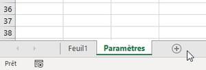
Click at the bottom of the window on the + sign to create a new sheet in your Excel workbook. Then double-click on the Newly added Sheet2 tab, in order to rename this sheet by calling it, for example, Parameters.

It is then possible to hide your Parameters sheet by clicking on it with the right mouse button, choice Hide. To redisplay it, right-click any other sheet name (for example Sheet1) to choose Pin up… and see the list of hidden sheets.

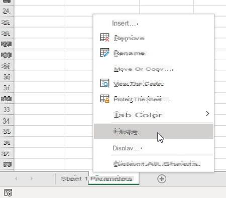
By right-clicking on the name of a sheet, you can also Protect the sheet, including password.
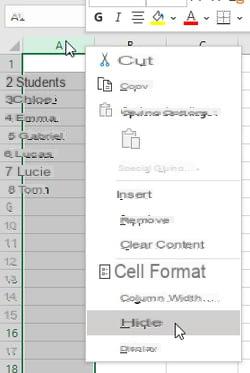
If you are not very comfortable with handling multiple sheets and prefer to work with a single worksheet, you can enter the items and then hide the column. Right-click on the column letter at the top of the sheet (on the letter A in the example below), and choose Hide from the context menu. To redisplay the hidden column, select the surrounding columns, right-click on them to display the context menu, and choose Show.

The labels that will appear in the Data validation list can appear either in a column or in a row, as desired, but the cells must imperatively be adjacent, and therefore follow each other.
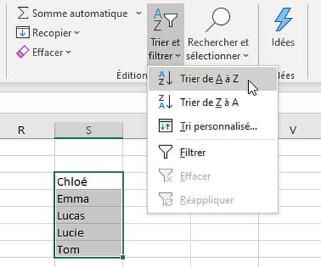
The data in your drop-down list will appear in the order it appears here, it will not automatically be sorted alphabetically. So sort them yourself if it can make typing easier: select the list and click the tab Home> Sort and filter> Sort from A to Z.

If the initial list contains duplicates to delete, select this list and click on the tab Data> Remove duplicates.

How to add item to an Excel drop-down list?

We have seen that in certain cases, with Excel tables in particular, it suffices to type a new value at the end of the source list so that it is added to the drop-down list. Otherwise, depending on how your dropdown refers to the source cell list, here's how to add an item without having to change the Data Validation options ...

Add item to a defined drop-down list from a range of cells

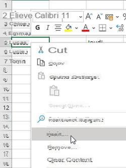
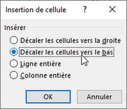
To later add an item to the drop-down list, right-click inside the list, choose Insert… and Shift cells down and enter the new element in the cell that is added. Remove your list if necessary.

Other method: in the area Source of Data validation, if you initially select a range of cells larger than necessary to later add empty cells to the end of the list, this will allow you to expand the list without having to redefine the data validation drop-down lists that refer to it . Corn…

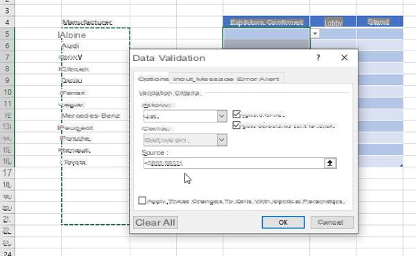
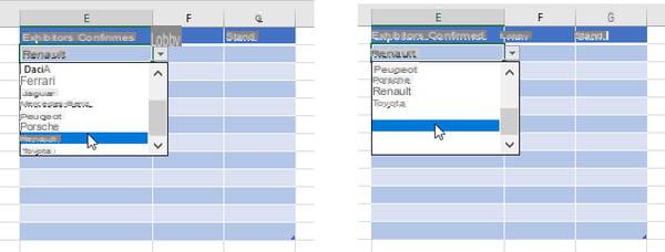
... We found that while the lines containing the empty cells (lines 17 to 21 in the example above) do not have never content neither data nor formatting (bold, italics, frame…), Excel does not show empty choices in the drop-down list, that's perfect. Otherwise, it adds empty items at the end of the drop-down list: the list remains usable but it is not very elegant as seen below ...

Add item to a defined drop-down list from a named range

To add an item to the drop-down list that displays the contents of a named range, do the same as for a range of cells (see above): right-click on one of the cells in the named area (but not the first), select Insert> Shift cells down then type the new item in the empty cell. Sort the list again if necessary.

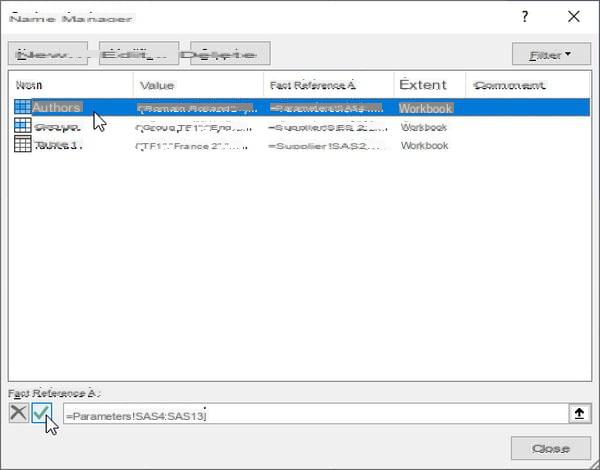
In Excel for Windows, if you want to redefine the scope of a named range of cells, click on the ribbon tab Packages, then below on Name manager. Click the name of the range, then click below in the box Refers to to select a new range in the sheet. Finally click on the green tick to validate and press the button Close. Note that this window is also used for Edit (add a comment, for example) or Remove a named range.

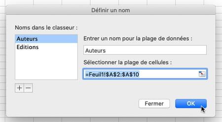
In Excel for Mac, to redefine the extent of a named range, click the tab Packages then Define a name (or in the menu Insert> Name> Define name). Click on the name, redefine the range of cells and press OK. + and - buttons allow you to create or delete names.

How to delete an item in an Excel drop-down list?

To avoid having to reconfigure your drop-down list via the Data Validation dialog box, here's how to do it.

Go to the sheet where the initial list is located.
Right-click on the cell you want to remove from the source list.
Click on Remove in the context menu.

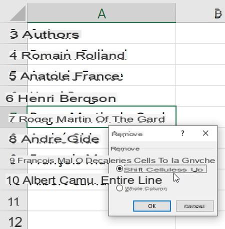
In the small Delete dialog box, check the box Shift cells up and press the button OK. If the data is arranged in a row and not in a column, check the box instead. Shift cells to the left.

How to delete drop down list in Excel worksheet?

It is of course entirely possible to delete drop-down lists that we no longer use in a spreadsheet, without erasing the content of cells filled with the list.

Select at least one cell in which the drop-down list is displayed or only the affected cells.
Click on the tab Data> Data validation.

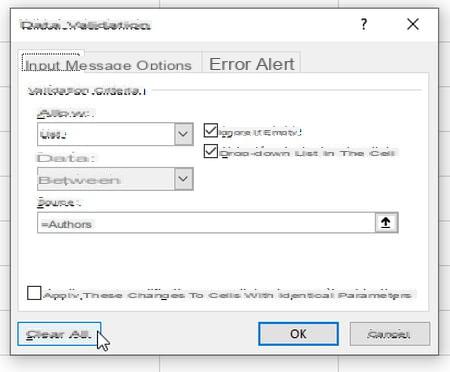
Under the tab Tools, if you want all cells with the same data validation options to be affected, so all cells displaying this drop-down list: check the box Apply these changes to cells with identical settings.
Click on the button Reset all.
The drop-down list will no longer appear, but the content of already filled cells is not deleted.
If you don't know where the cells that contain data validation are located, on the Home, click on the far right of the ribbon Search and select, And then Data validation.

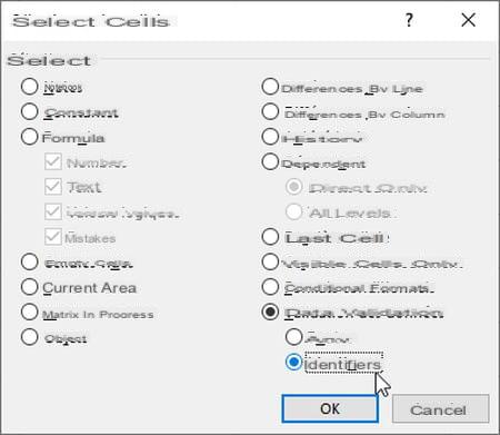
Before clicking on Search and select, if you have selected a cell containing a drop-down list, click Select cells> Data validation> Identical : Excel selects all cells showing the same drop-down list. You still have to go to the tab Data> Data validation> button Reset all.

How to add help message in Excel drop down list?

Sometimes it is useful - even desirable! - display a message in the form of a bubble to help the users of a sheet to correctly use a drop-down list.

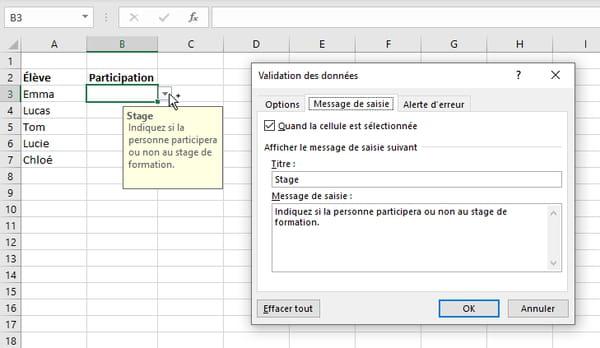
In the window Data validation, tab Input message, in the Title (30 characters maximum) and Input message (250 characters) boxes, specify the information that will be displayed in the form of a tooltip.
Uncheck the box When the cell is selected to temporarily or permanently deactivate this option.

How to control the entry and display an error message in an Excel drop-down list?

Always to help the users of your sheet, it is strongly recommended to carry out an entry control and to display an alert message when an error is detected.

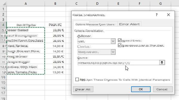
If you do not want to check the value entered in the cell, open the tab Error alert and uncheck the box When invalid data is typed.

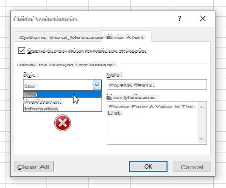
If, on the contrary, you wish to verify the entry, open the tab Error alert and leave the box checked When invalid data is typed.
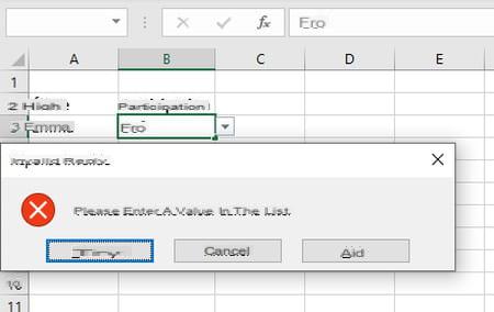
In the Style list, the choice Stop ( Stop, in older versions of Excel) displays an error message and rejects any incorrect value entered.

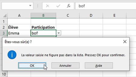
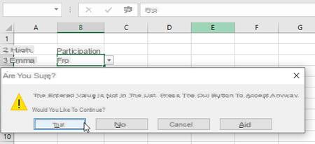
In the Style list, the choice Disclaimer displays an error message but allows the user to accept the entered value anyway even if it is not in the list. This is what we have indicated in the Title and Error message fields.

In the Style list, the choice Information is quite similar to the choice Disclaimer : it displays a message and this time offers a button OK to validate a value not provided for in the list. We have therefore adapted the message to be displayed in the fields Title et Error message.