➤Excel pivot table: example, create, update ... 🕹

Do you have large lists of data and want to summarize them in a report? Or analyze them according to different points of view and search criteria? Excel contains a tool specially dedicated to these tasks: the pivot table!

When working with large amounts of data, it is common to want to synthesize it, whether to obtain a global and quickly understandable view of a set of values or, on the contrary, to study a subset more precisely. meeting specific criteria.

You could of course take the time to sort, filter and then manually roll up your valuable data into a new table that meets your needs. However, every time you add or remove data from your initial list, you will run the risk of your destination table "forgetting" them and you will have to regularly check your calculation formulas to avoid this. In addition, if you want to group and summarize your data according to different criteria, then you will have to manually modify the structure of your destination table, or even create several summary tables if you want to maintain different points of view on your data. These manipulations will quickly prove to be tedious and a source of error.

Fortunately, Excel's PivotTable tool lets you accomplish all of these tasks with just a few clicks and without typing any formulas. In order to present to you the different notions necessary for the use of pivot tables, this practical sheet is accompanied byan example workbook, downloadable for free here. All the operations described in this guide are based on this file: we therefore strongly recommend that you use it in parallel with your reading.

Download a sample pivot table for Excel

This sheet was produced with the Office 2019 version of Excel. However, all the functions presented are available identically in the Office 2016 and Microsoft 365 (ex-Office 365) versions of Excel, with the exception of the creation of custom PivotTable styles which is not offered. in the web version of Microsoft's spreadsheet.

Why use a pivot table?

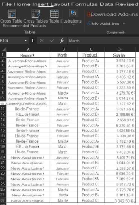
You are working on a large list of data, for example a sales journal, and you want to quickly know the sum of the elements of this list by grouping them simultaneously according to several criteria, for example by product category and month of sale. In this case, using a pivot table will allow you to quickly get this result, choose how the summary data will be arranged, and instantly change this layout whenever you need to. The diagram below illustrates how a PivotTable synthesizes data and organizes it visually.

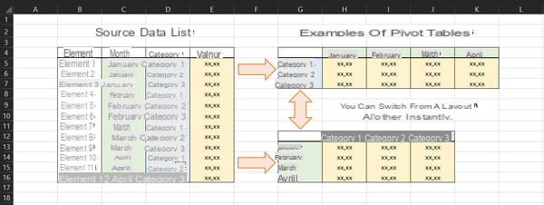
Excel pivot table: example, create, update ...

We speak of a “crosstab” because the categories used to group the data can be broken down into both rows and columns. On the example of a pivot table at the top right of the image, the yellow cell at the "intersection" of the "January" and "Category 1" fields returns the sum of all the items in the initial data list that contained the "January" and "Category 1" values in the "Month" and "Category" columns. In this case, a single item meets both of these criteria, but the data list could contain thousands of items which would then be processed automatically by the PivotTable, without you needing to sort or filter the data in prior.

We also speak of a "dynamic" table because, on the one hand, its layout can be changed instantly via simple operations with the mouse or keyboard and, on the other hand, any addition, modification or deletion of data in the initial list. is automatically taken into account in the result of the groupings.

How to create a pivot table with Excel?

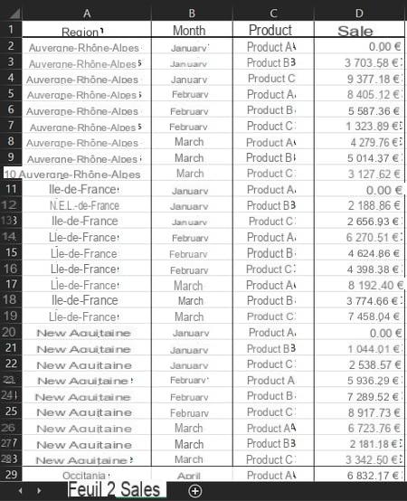
Before you generate a PivotTable, you must ensure that the data in your initial list meets the following prerequisites:

The data in the same column must all be of the same type (number, date, text, etc.).
The first row of your data list should contain the column headers.
Your list should not contain any merged cells.
Your list should not contain empty cells (Excel is able to recognize and handle empty cells if they exist, but it is best to avoid them as much as possible).

Once these conditions are met, you can start creating your PivotTable.

Click somewhere in the data list, then, in the tab Insertion on the ribbon, click Pivot table.

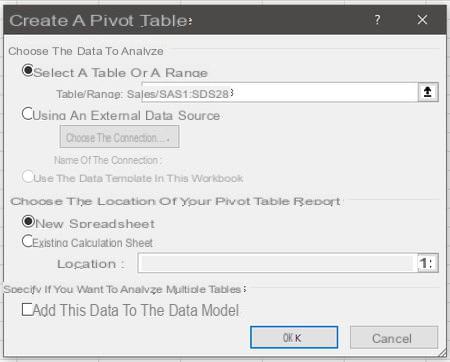
In the Create PivotTable dialog box, verify that the field Table / Beach does contain the references of the data list. By default, if you clicked somewhere in the list correctly and it does not contain blank cells or merged cells, Excel correctly determined its size. If not, click up arrow icon to the right of the field Table / Beach and manually select the entire data list.
In the Choose a location for your PivotTable report section, verify that the New spreadsheet is checked. You can of course tick the box Existing spreadsheet and manually select a location in the same sheet as the data list, but the readability of the whole may be less good.
Validate the creation of the pivot table by clicking on the button OK of the Create PivotTable dialog box.

A new worksheet is inserted by Excel into the workbook and a pane named PivotTable Fields appeared on the right of your screen.

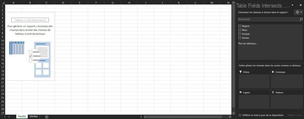
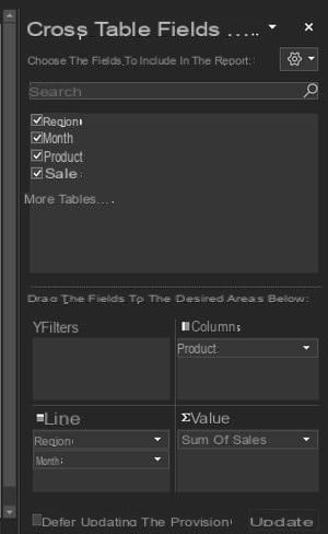
The PivotTable Fields pane consists of five frames. The first shows you the list of available data fields, which corresponds to the column headers of the initial data list. The other four frames represent the zones of the pivot table: it is by moving the available data fields in the different zones that you are going to create the PivotTable layout.
In the list of available data fields, check the boxes to the left of the words Region, Product et Sales. A PivotTable has appeared in your worksheet, and if you look at the bottom four frames, you will see that the words Region et Product have been added in the area lines and that the words Sum of Sales appeared in the area Valeurs.

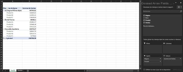
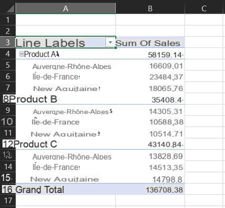
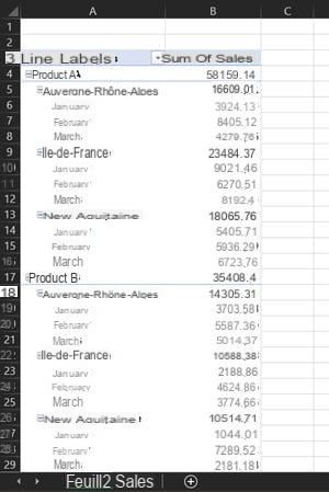
At this point, you've created a pivot table that groups your data by region then by product name and has a subtotal for each category as well as a grand total at the bottom of the table. You will also find that the categories in the PivotTable are arranged in the same order as the data fields in the frame. lines in the Available PivotTable Fields pane. Remember this principle, it is the heart of the organization system of a pivot table.

In the frame lines in the PivotTable Fields pane, click the gray arrow to the right of the name Region and, in the contextual menu that appears, click on Go down, or left-click and hold on the name Region and bring it down under the name Product before releasing the mouse button.

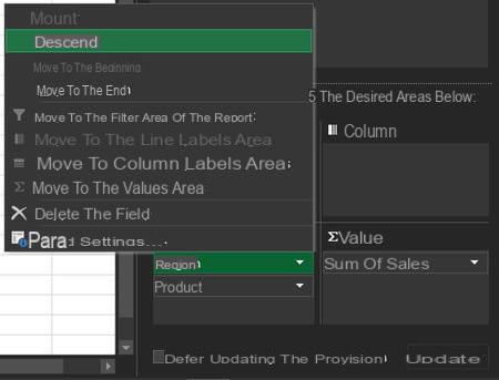
In the frame lines, the name Product is now in first position and the name Region in second. On the PivotTable side, you will find that the order of the data groupings and subtotals has also reversed.

This simple manipulation gives you an overview of the power and flexibility of a pivot table. In seconds, you've got a whole new perspective on your data without needing to sort or rearrange it in the original list.

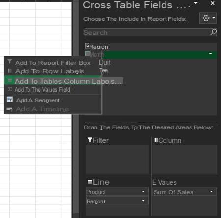
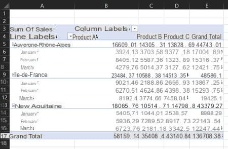
In the Available PivotTable Fields pane on the right of your screen, in the upper frame, right-click on the name Month then select Add to column labels, or left-click and hold on the name Month and move it to the area Columns before releasing the mouse button.

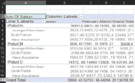
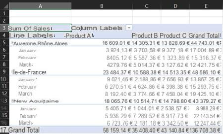
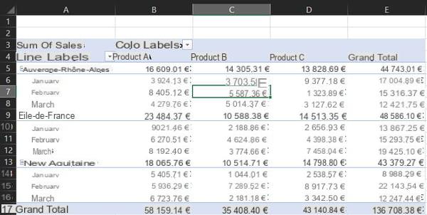
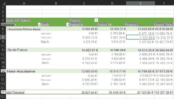
In the spreadsheet, the pivot table has expanded to three additional columns and now shows, in addition to subtotals by product name and region, monthly subtotals for each of these categories as well as a grand total to the right of the table.

At this point, you have created a complete pivot table: from a list of data organized in rows, you have obtained a summary report that groups your data into categories, divides them into rows and columns and displays them. subtotals. Try changing the distribution of categories between rows and columns to understand how Excel changes the PivotTable.

In the Available PivotTable Fields pane, use the mouse to pass the name Month of the area Columns to the area lines, in the last position after the names Product et Region, then pass the name Product of the area lines to the area Columns and observe the changes that occur at each step in the PivotTable.

How to format a pivot table with Excel?

To make your PivotTable easier and more enjoyable to read, especially when it has a large number of categories and data, Excel offers (very) many formatting options. For example, you can choose a different layout for categories, custom number formats for the values area data, colors for headers and borders, and much more.

How to change the number format of values?

You will notice that the data in the area Valeurs of the PivotTable appear as numbers with two decimal places, without a thousands separator, which is not very readable for currency values. You can choose to display this data in any number format available in Excel.

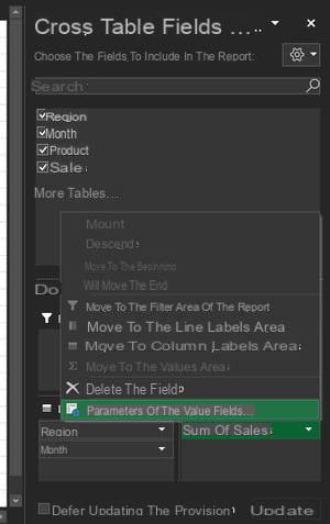
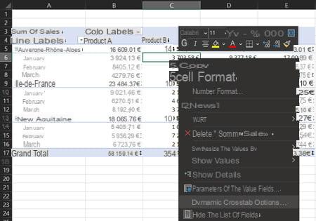
In the Available PivotTable Fields pane, in the Valeurs, click on the name Sum of Windes then Parameters of value fields.

In the Settings dialog box for value fields that opens, click the button Number Format.

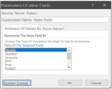
The dialog box Cell Format opens. In it, you can select any existing cell format in Excel or create a custom format by clicking the category custom. In this case, click on the category Monetary then validate your choice by clicking on the button OK at the bottom right of the dialog box.

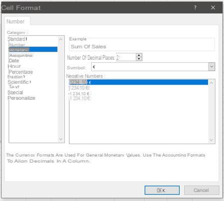
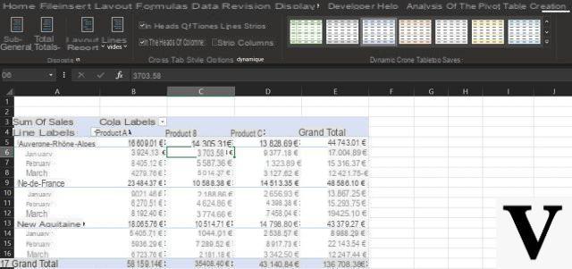
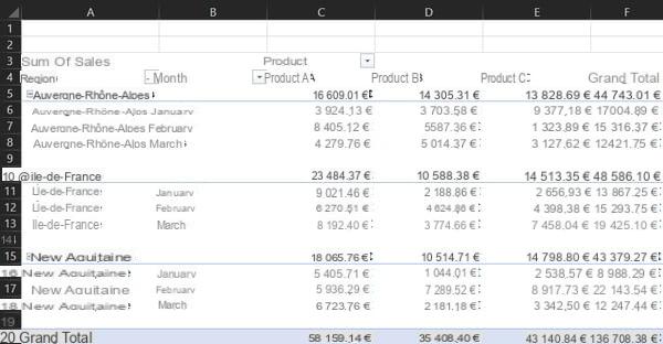
Back in the Value Fields Parameters dialog box, click the button OK at the bottom right to apply your change to the PivotTable. Zone data Valeurs are now displayed as currency values, with a thousands separator, two decimal places, and the € symbol.

How to change the width of the columns?

When creating a pivot table, the width of the columns automatically adapts to the content of the cells, which may not give the desired result if, for example, you want all the columns to have the same width. Fortunately, it is very easy to manually change the width of the columns and keep it during PivotTable updates.

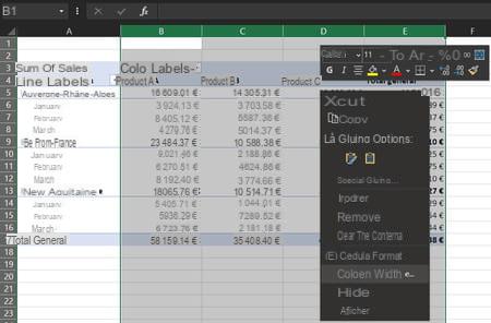
To give the same width to several columns, select the ones you want to modify by clicking on their label (the letters A, B, C, D, etc., located above the first row of the worksheet). For example, left-click and hold on the column label B, move your cursor to the column label E then release the left mouse button. All columns of B à E are then selected.

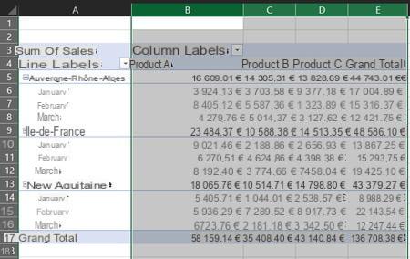
Then move your mouse over the separator line between the column labels E et F until the cursor changes to a double black arrow. Then do a left-click and hold and move your cursor to the right to increase the size of the columns or to the left to reduce it. When you release the left mouse button, all previously selected columns assume the same width.

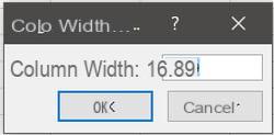
Alternative method: select the columns whose width you want to change by clicking on their label (as explained above), right-click anywhere in the selection area and then choose Column width from the context menu. A Column Width dialog box opens in which you can directly enter a number to define the width of the selected columns. This method is more precise, but less intuitive than the previous one.

Once you have assigned the desired widths to your columns, it is necessary to go through the options of the pivot table so that these settings are kept when updating the table. Indeed, by default, Excel automatically adjusts the width of columns to their content when refreshing the PivotTable. Fortunately, this option can be changed with just a few clicks.

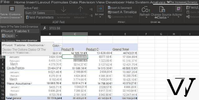
In the worksheet, click anywhere inside the PivotTable. This brings up the tab Pivot Table Analysis in the ribbon. Click on it, then on the menu PivotTable options and finally on the button Options.

You can also right-click in any cell of the PivotTable and, in the context menu, click PivotTable options.

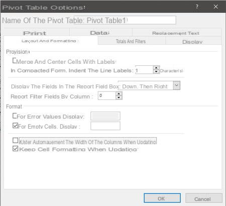
With either of the methods described above, the PivotTable Options dialog box appears on your screen. It has several tabs and opens by default to the one titled Layout and formatting. That's good, it is the one that interests us in this case. Find the box Automatically adjust column width when updating and uncheck it. Take the opportunity to check that the box Keep cell formatting when updating, just above, is checked. This way, you can be sure that all the formatting that you have applied manually will be preserved when refreshing the PivotTable.

How to change the style and layout of the pivot table?

There are lots of possibilities in Excel to change the way the PivotTable visually organizes your data, such as showing grand totals for rows and columns, where subtotals are located, or how data categories are nested. Microsoft's spreadsheet software also lets you choose from a list of ready-made (and pretty elegant for the most part) table styles that can be instantly applied to your PivotTable, saving you the hassle of formatting. to let you focus on the substance. And, if none of the predefined styles meet your expectations, it is quite possible to create your own which will then be available for all your future PivotTables. Note that creating custom styles is not available in the web version of Excel. On the other hand, if you created a custom table style in a file on a desktop version of Excel, and then open that file on the web version, your custom style will be present and usable, but not editable.

In the worksheet, click any cell in the pivot table to bring up the tab Creation in the ribbon, then click the ribbon. This tab has three sections: Layout, PivotTable Style Options, and PivotTable Styles.

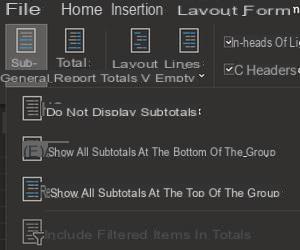
In the Layout section, the button Subtotals allows you to choose between three display options, the name of which is quite self-explanatory: Do not display subtotals, Show all subtotals at the bottom of the group et Show all subtotals at the top of the group (this is the option enabled by default). Try each of them to see how the PivotTable changes in appearance, then switch the display back to subtotals at the bottom of the group before moving on. A final option called Include filtered items in totals appears at the end of the list but it is inactive for the moment because you have not applied any filter to your PivotTable. As its name suggests, it allows you to include in the subtotals the value of data hidden by a filter, which can lead to errors in reading and interpreting the results of a PivotTable. To be used with caution therefore.

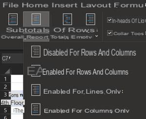
Still in the Layout section, the button Grand totals offers four display possibilities: Disabled for rows and columns, Enabled for rows and columns, Enabled for rows only et Enabled for columns only. Again, give it a few tries and then come back to the option Enabled for rows and columns before moving on.

The next button in the Layout section is called Report layout. It allows you to choose how Excel organizes the categories of data that you have placed in the box lines of the pivot table.

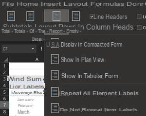
The first option, Show in compacted form, is the one used by default and therefore the one you see from the beginning. In this display mode, the data categories of the zone lines are grouped into a single column and displayed as a tree structure, with a right indent applied to each subcategory and a subtotal for each category that can be displayed at the top or bottom of the group (see previous section of this practical sheet). This arrangement offers the advantage of optimizing the space occupied by the categories in width and therefore of leaving more room for the display of values. Its drawback is that it groups the filters applicable to the different categories in a single button (present in cell A4 in our example), which can make filtering on several categories less readable. This aspect will be developed later in this practical sheet.

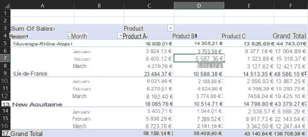
The second option available, View in Outline View, is quite similar to the previous one: the data categories of the zone lines are always displayed as a tree structure and a subtotal for each category can be displayed at the top or bottom of the group. However, the categories of the area lines are this time spread over several columns, one column per category to be more precise. This mode therefore uses more space in width for the display of categories and can give an impression of "mess" with the empty zones in each group. However, as each category has its own column, this mode offers the advantage of assigning a filter button to each category, which makes filtering on several criteria very readable.

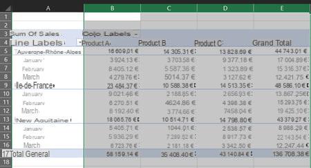
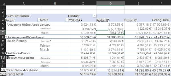
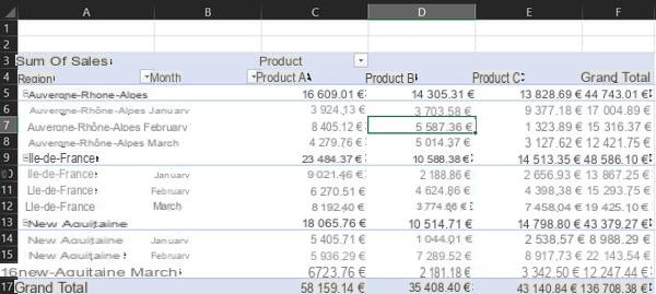
The third and final option is called View in tabular form. This time, the categories of the area lines are no longer displayed in the form of a tree structure but in the form of a classic table and, crucially, the subtotals must be found at the bottom of each group. As in the display in Plan mode, each category of the zone lines is distributed in an individual column and therefore offers its own filter button.

Finally, the button Report layout gives you two additional options: Repeat all element labels ou Do not repeat item labels. These two options actually control a single parameter, allowing it to be enabled or disabled. By default, repeating item labels is turned off, which is why you see empty spaces in each category group. If you click on the option Repeat all element labels, then the name of each category will be repeated in its column until the next group. This can be useful if a category has a lot of items and its length exceeds the display height of your table. Note that this option does not work in display in compacted form.

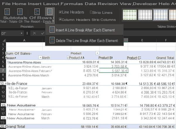
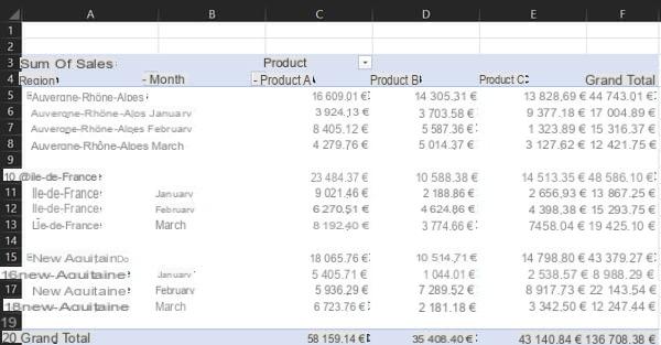
The Layout section has a final menu called Empty lines which contains two options: Insert a line break after each element ou Remove line break after each item. The first option inserts a blank row after each group of categories, which can be useful to air your PivotTable, especially if you have opted for the repeating item labels. The second option simply removes the empty lines inserted by the first.

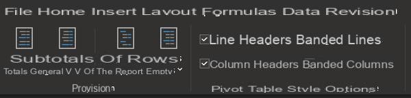
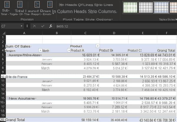
The next section of the tab Creation on the ribbon is named PivotTable Style Options, and contains four checkboxes each allowing you to enable a specific formatting option. By default, the options Row headers et Column headers are checked and the options Strip lines et Band columns are unchecked.

If you uncheck the box Row headers, the formatting of the first row of each category group will disappear.

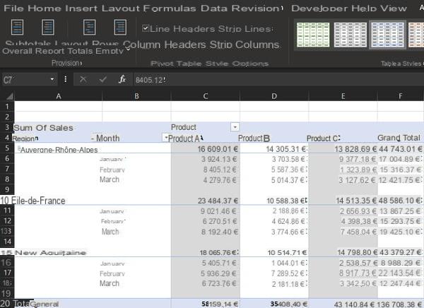
If you uncheck the box Column headers, it is the formatting of the column headers of the pivot table which then disappears.

The houses Strip lines et Band columns produce different effects depending on the applied pivot table style. You'll see how to choose a table style later in this how-to, so feel free to toggle these options on and off after a style change to see how they affect table formatting. In general, the options Strip lines et Band columns make it easier to distinguish between rows and columns, by showing separator borders or by applying alternate row or column formatting. Try toggle these options on and off to see the result on the current table style.

The last part of the Tab Layout section Creation is entitled PivotTable styles and contains the famous ready-made table styles that you can instantly apply to your PivotTable.

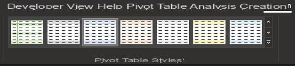
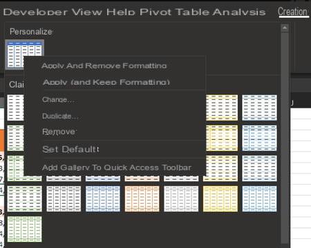
The PivotTable Styles section gives you a first sample of the available table styles, but there are many more: click on the arrows to the right of the sample to scroll through the available styles or on the arrow topped with a line to display a drop-down list of all existing styles. By hovering over the table styles with your mouse, without even having to click on them, you will see that Excel temporarily applies the formatting to the PivotTable, which is very useful for quickly comparing the various possibilities available to you. .

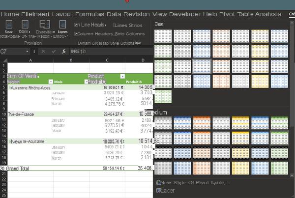
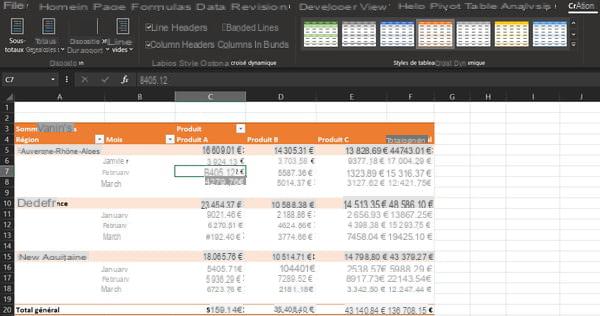
To permanently apply the table style you like, simply click on it in the drop-down list, the corresponding formatting will then apply to the entire PivotTable. You can of course change the table style as often as you like by simply repeating the previous step.

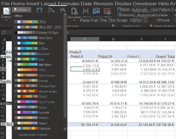
Note that the styles offered are dependent on the color scheme used in your Excel workbook, and if none of the table colors offered are suitable for you, you can get new ones by changing the color scheme through the tab Layout ribbon, Themes section, menu Colors.

If, despite everything, you do not find what you are looking for among the multitude of table styles offered, it is possible to create completely personalized styles. Please note, as explained previously, this function is not available in the Web version of Excel.

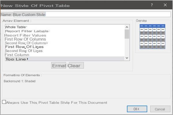
In the tab Creation, in the PivotTable Styles section, display the list of available styles by clicking the arrow topped with a line then, below the list, click on New PivotTable Style. A dialog box with the same name opens.

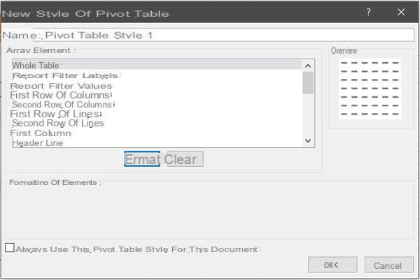
In the field Name, you can give your PivotTable style a custom name. Then things get a bit more complicated. Each entry in the Table Items list represents an area of the PivotTable that can be given special formatting. You must therefore configure each element individually until you get the desired result, which may take more or less time depending on the complexity of the table style you want to achieve.

To change the formatting of a table area, click its name in the Table element list, for example on Header rows, then the button Size under this same list. A Format Cells dialog box opens. It contains three tabs, Police, border et Filling, which allow you to set various formatting settings. They work exactly the same as when formatting cells directly in a worksheet. Experiment and apply different formatting then click on the button OK at the bottom right of the Format Cells dialog box. Repeat the operation several times with other entries in the Table item list. When you're done, look at the Preview section to the right of the New PivotTable Style dialog box. As the name suggests, it gives you a preview of the formatting that will be applied by your custom table style.

If you are satisfied with the result, click on the button OK at the bottom right of the New PivotTable Style dialog box to save your custom style. It will now be available in the list of PivotTable styles tab Creation tape. You can of course modify, duplicate or delete it with a simple right-click on it.

The number of table elements that can be customized is quite large, and it will probably take you some time to fully understand which area of the PivotTable each corresponds to. Do not hesitate to save a personalized style that you will evolve over time by testing it on the different pivot tables with which you work. Excel's creative potential is immense and (almost) only limited by your imagination and experience.

How to sort and filter a pivot table in Excel?

Like any range of data organized as a table in Excel, a pivot table can be sorted and filtered automatically using tools provided for this purpose. In terms of sorting, we find the classic functions of ascending, descending and personalized sorting. On the filtering side, auto-filters and segments are present as well as a filter area specific to pivot tables, which can be used for more readability.

How to sort data in a pivot table?

First solution: use the auto-filters. Click on the white button containing a black triangle which is to the right of the header cell of the column by which you want to sort your data, for example column Region. A context menu appears. The first two options allow you to sort your data in ascending or descending order (from A to Z or from Z to A in the case of a column containing text).

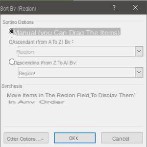
You can also choose to use Additional sorting options. These additional options will be different depending on the data type of the column (text, number, date, time). In all cases except for the numbers, you can choose to sort your data manually by dragging and dropping using the mouse.

Second solution: right-click on a cell of the PivotTable containing a data, it does not matter whether it is a category or a value, and in the context menu that appears, click on Trier then choose your sorting option as before.

How to filter data in a pivot table?

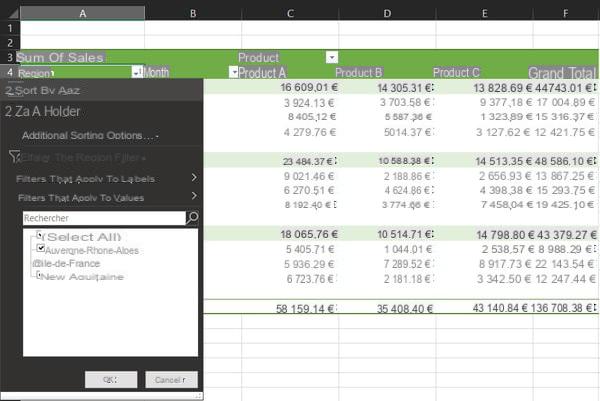
As with sorting, the most intuitive and straightforward method is to use auto-filters. Click on the white button containing a black triangle which is to the right of the header cell of the column by which you want to filter your data, for example column Region. A context menu appears.

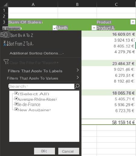
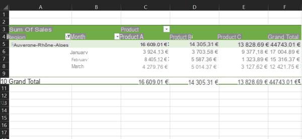
In the second half of this menu, a list of checkboxes allows you to select the data to show or hide, by simply checking or unchecking the corresponding box. For example, uncheck the boxes Ile-de-Spain et New Aquitaine then validate by clicking on the button OK at the bottom of the menu. PivotTable now only shows region data Auvergne-Rhône-Alpes.

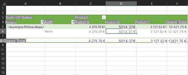
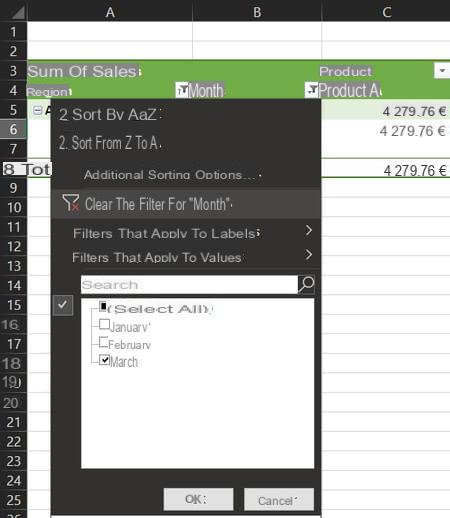
You can combine the filter criteria on several different categories. For example, open the auto-filter of the column Month and in the list of checkboxes, uncheck those corresponding to the months of January et February, then validate this filtering by clicking on the button OK. PivotTable now displays region data Auvergne-Rhône-Alpes of the month of March only.

To remove the filter criteria applied to a column, open the auto-filter for the column in question and click on Clear filter. Repeat this for each column for which you want to remove filtering.

Second method: use the specific filters area of the pivot table. Click somewhere in the PivotTable so that the PivotTable Fields pane appears on the right side of the window. Choose one of the categories present in the zones lines ou Columns, click on it then select Move to the Filter area of the report from the context menu. You can also move the chosen category from its current zone to the zone All filter brewing methods by dragging and dropping using the mouse.

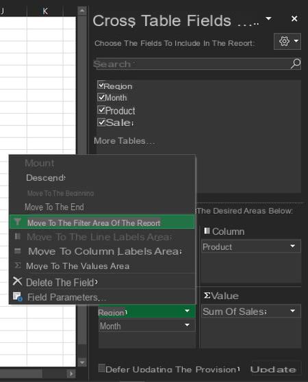
For our example, first drag the category Region of the area lines to the area All filter brewing methods, then the category Product of the area Columns to the area All filter brewing methods.

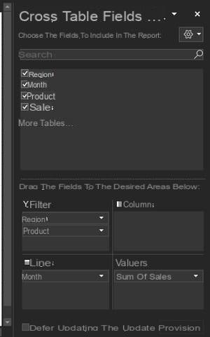
You will see that the structure of the PivotTable has changed: the subtotals by region and by product have disappeared from the table, and two rows have appeared above that correspond to the PivotTable filters. They each contain an auto-filter which works like those seen previously, but in a slightly simplified way.

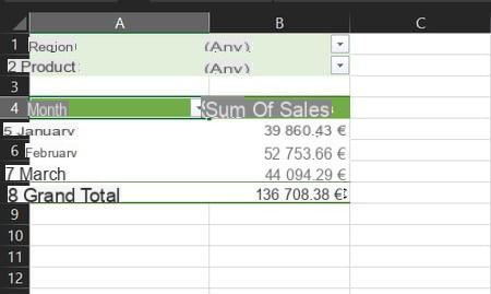
Click on the auto-filter in the row titled Region, a context menu will open in which you can select one of the entries of this category. By default, you can only select one entry from the list. By checking the box Select multiple items at the bottom of the list, you can then make a multiple selection. However, this type of filtering with several criteria within the same category is not recommended in this display mode, as we will illustrate just below. There is a tool more suitable for filtering with multiple criteria (segments) that we will see later in this practical sheet. For our example, open the auto-filter of the row Region, select the element Ile-de-Spain and validate by clicking on the button OK, then open the auto-filter of the line Product, select the element Product A and validate by clicking on OK.

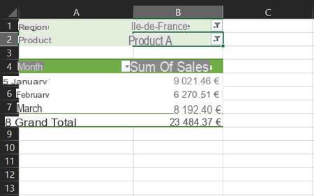
PivotTable now only displays values for categories Ile-de-Spain et Product A and the filtering criteria used are clearly visible above the range of the table, which greatly facilitates reading and avoids data interpretation errors when performing several successive filterings. If you had checked the option Select multiple items in the previous step, and had carried out a filtering with several criteria in the same category, then the filter line would have displayed "Several elements" instead of the precise name of the filtering criterion. This would require you to reopen the filter list periodically to remember which criteria are applied.

Use of the area Filters of the pivot table, rather than the classic auto-filters present in each column, is therefore particularly useful for working on specific subsets of a list of data comprising many categories.

Finally, a third method, which will combine the advantages of the previous two, namely displaying the subtotals of all the categories in the pivot table and permanently displaying the criteria used in the event of multiple filtering: the segments. Start by reverting to the previous structure of the PivotTable. In the PivotTable Fields pane, bring back the category Region in first position in the area lines and the category Product in the zone Columns.

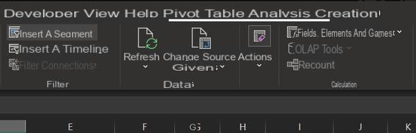
Click any cell in the pivot table to bring up the tab Pivot Table Analysis in the ribbon and click on it. In the Filter section, click the button Insert segment.

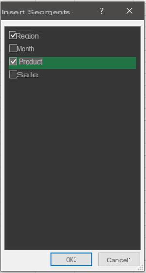
A dialog box titled Insert Segments opens. It contains the list of categories of your PivotTable in the form of check boxes. For our example, check the boxes Region et Product then validate your selection by clicking on the button OK at the bottom of the dialog box.

Two objects appeared in the worksheet, above the pivot table. These are the famous segments Excel, very practical and ergonomic visual filtering tools. First, using the mouse, drag and drop them to the right of the pivot table so as not to hide it.

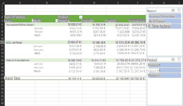
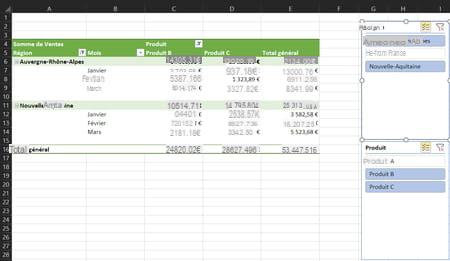
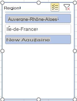
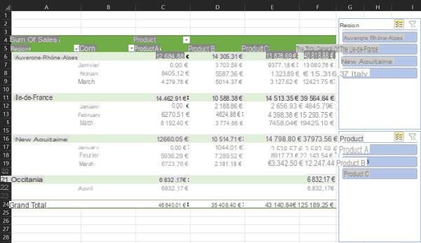
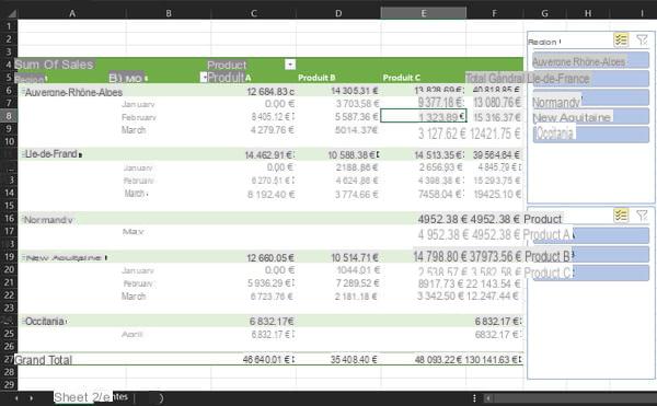
Segments work the same as auto-filters, allowing you to choose which categories to show or hide by simply clicking on their name inside the list, but with the difference in size that the segments will remain visible. permanently. In the segment Region, click on the icon representing a validation list to the right of the name "Region" to activate multiple selection, then click on the items Auvergne-Rhône-Alpes et New Aquitaine. In the segment Product, activate the multiple selection as before, then click on the elements Product B et Product C. The pivot table instantly adapts to your changes and the filter criteria used remain visible at all times in the segments. You can obviously change your filters by simply clicking on the corresponding elements in the segments.

To clear filters applied using segments, click funnel and red cross icon in the header of the relevant segment.

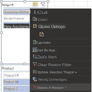
To completely delete a segment, right-click on it and select To delete " ... ".

How to refresh a pivot table with Excel?

Another advantage of PivotTables is that they can be updated instantly when changes are made to the initial data list. Whether you've added, edited or deleted rows, or even added columns representing new categories, it's possible to refresh the PivotTable with just a few clicks.

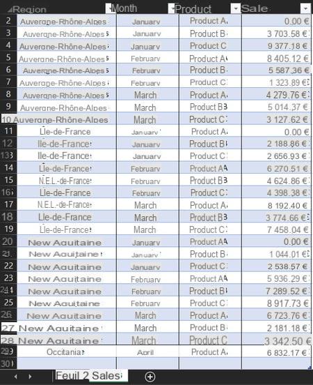
Make some modifications in the initial data list: replace some values with a zero and add a line at the end of the list with new entries for the categories Regions et Month, for example "Occitanie" and "Avril".

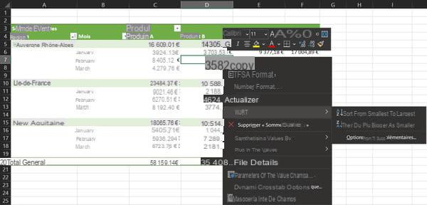
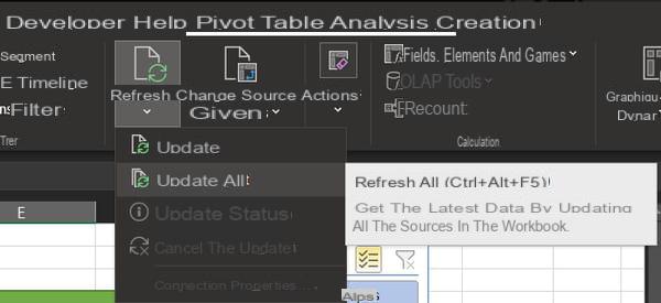
Return to the worksheet containing the PivotTable and click any cell in the PivotTable to bring up the tab Pivot Table Analysis in the ribbon, then click the ribbon. In the Data section, click the button actualize then Refresh all. You can also right-click on a pivot table cell and choose actualize.

The pivot table has updated: the values clearly show the amounts you modified in the initial data list (the zeros). However, the row added at the end of the list does not appear because it is outside the range of data on which the PivotTable is based. Don't worry, it's very easy to change the source data range and even set it to automatically expand every time you add a row or column.

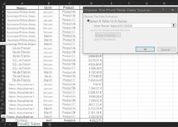
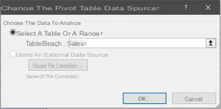
In the tab Pivot Table Analysis, in the Data section, click the button Change the data source. Excel takes you back to the sheet containing the original data list and opens a dialog box named Edit PivotTable Data Source. You can directly enter the references of the data source in the field Table / Beach using the keyboard or select the range in the sheet using the mouse. Validate the modification of the range by clicking on the button OK at the bottom of the dialog box.

You automatically return to the sheet containing the pivot table which, this time, shows a new category named Occitania and a subcategory named April.

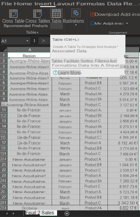
To avoid having to change the source data range manually each time you add a row or column, the best way is to convert the data range to structured table. To do this, go back to the worksheet that contains the source data range and select it in full. Then click on the tab Insertion ribbon then on the button Table.

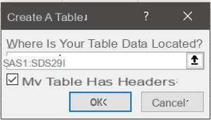
The Create Table dialog box opens. Check that the references contained in the field Where is the data for your table located? cover the entire source data range and that the checkbox My table has headers is checked, then validate by clicking on the button OK.

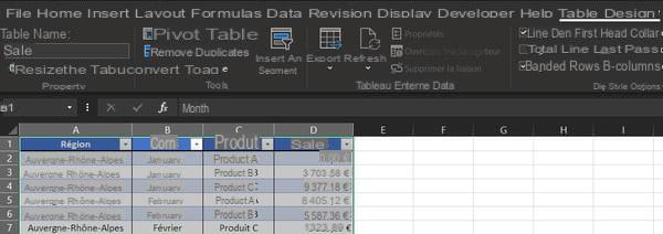
The data list then changes appearance. Above all, it has become a structured table which has several advantages: it can be referenced by a name rather than by its address, and the additions of rows and columns will be automatically taken into account in its scope. Before moving on, assign a name to this structured table: stay on the same sheet and click on the tab Table design in the ribbon, then in the field Painting name and give it a meaningful name, for example Sales.

Return to the sheet containing the pivot table, click on a cell of the latter, on the tab Pivot Table Analysis ribbon and, finally, the button Change the data source. In the Edit PivotTable Data Source dialog box, in the Table / Beaches, simply enter the name of your structured table, Sales in this case, and validate by pressing the button OK.

The pivot table is now linked to the structured table Sales. Any addition of row or column to this structured table will be taken into account when refreshing the pivot table.

Return to the sheet containing the structured table Sales and go to the last cell of the table (D29). Press the key tabulation on your keyboard. A blank row is added to the structured table, with the same formatting as the previous rows.

Fill this row with new data, for example "Normandy", "May", "Product C" and "4952.38". Then return to the sheet containing the pivot table, click on the tab Pivot Table Analysis ribbon, on the button actualize and Refresh all. The pivot table refreshes and shows a new category named Normandy and a subcategory named Mai.

Now you can add as many items as you want to your initial data list without worrying that they will be ignored when refreshing the PivotTable.

Pivot tables offer a multitude of other more or less sophisticated functions, making it possible to obtain more or less complex results. For example, they can display values not as sums but as percentages or differences from a base value from the original data list, and much more. However, these functions are beyond the scope of this practical guide for an introduction to the use of pivot tables. The concepts presented in this sheet nevertheless give you the knowledge necessary for the use of pivot tables which will meet the majority of cases that you may encounter.

Excel pivot table: example, create, update ...